Aircraft Delay Propagation Analysis with Big Data on AWS

Overview

Awarded Grade: A

• Presentation Slides

Developed as part of the IS459 Big Data Architecture module, this project explores how individual aircraft contribute to network-wide delay propagation across the U.S. air transport system. Flight delays are rarely isolated events; a single late arrival can ripple through the network, causing cascading disruptions that affect flights across the country.

By combining airline on-time performance data with FAA aircraft registration data, we sought to understand how tail-level behaviour, schedules, and operational patterns combine to create these cascading delays. The goal was to move beyond simple delay statistics and identify the specific "network multipliers"—aircraft that consistently amplify delays—and build a scalable analytics pipeline on AWS to predict them.

This work is part of a broader project that also examined airport-level congestion. However, this post focuses specifically on aircraft-level propagation and tail-level risk scoring. It uses the same core flight dataset but shifts the lens from the airport to the aircraft, analysing how individual planes carry delays from one leg to the next.

---

The Challenge

Which aircraft act as “network multipliers” for delays, and what can operations teams actually do about them?

The core of this analysis revolves around identifying persistent patterns of delay propagation. We wanted to answer a critical operational question: Which aircraft consistently turn a late arrival into a cascading series of departure delays?

To answer this, we needed to:

• Identify problematic aircraft that repeatedly propagate delays (the “network multiplier” effect).
• Quantify operational risk factors like turnaround time, fleet utilisation, and time of day.
• Build tail-level risk scores and clusters so ops teams can prioritise interventions on a small set of high-impact aircraft.

While the broader project also investigated airport congestion windows across major U.S. hubs (like ATL, ORD, JFK), this post focuses exclusively on the aircraft-level analysis and the AWS architecture that enabled us to track and predict delay propagation by tail number.

---

Data & Sources

Flight Operations

• Airline On-Time Performance dataset (1987–2008), containing nearly 120 million records with detailed flight-level timestamps, carrier codes, delays, origins/destinations and tail numbers.
• Flights are grouped by tail number to reconstruct aircraft-level itineraries and chains of consecutive legs.

FAA Aircraft Registry

To understand aircraft characteristics, we ingested the FAA’s releasable aircraft registry:

• MASTER: registration records keyed by tail number (N-number).
• ACFTREF: reference table mapping make/model/series codes to human-readable aircraft types.

These were joined to attach age, manufacturer, and model to each tail number for downstream analytics like “Does aircraft age drive cascading?” and “Which models cascade chronically?”.

Note on Weather Data

For the airport congestion part of the project, we built a separate enrichment layer using AWS Lambda and the Open-Meteo API to correlate delays with weather conditions.

However, the aircraft-level analysis detailed in this post is largely weather-agnostic. Instead of external weather factors, it focuses on internal operational patterns (turnaround times, schedules) and tail-level characteristics backed by the FAA metadata.

---

Architecture & AWS Stack

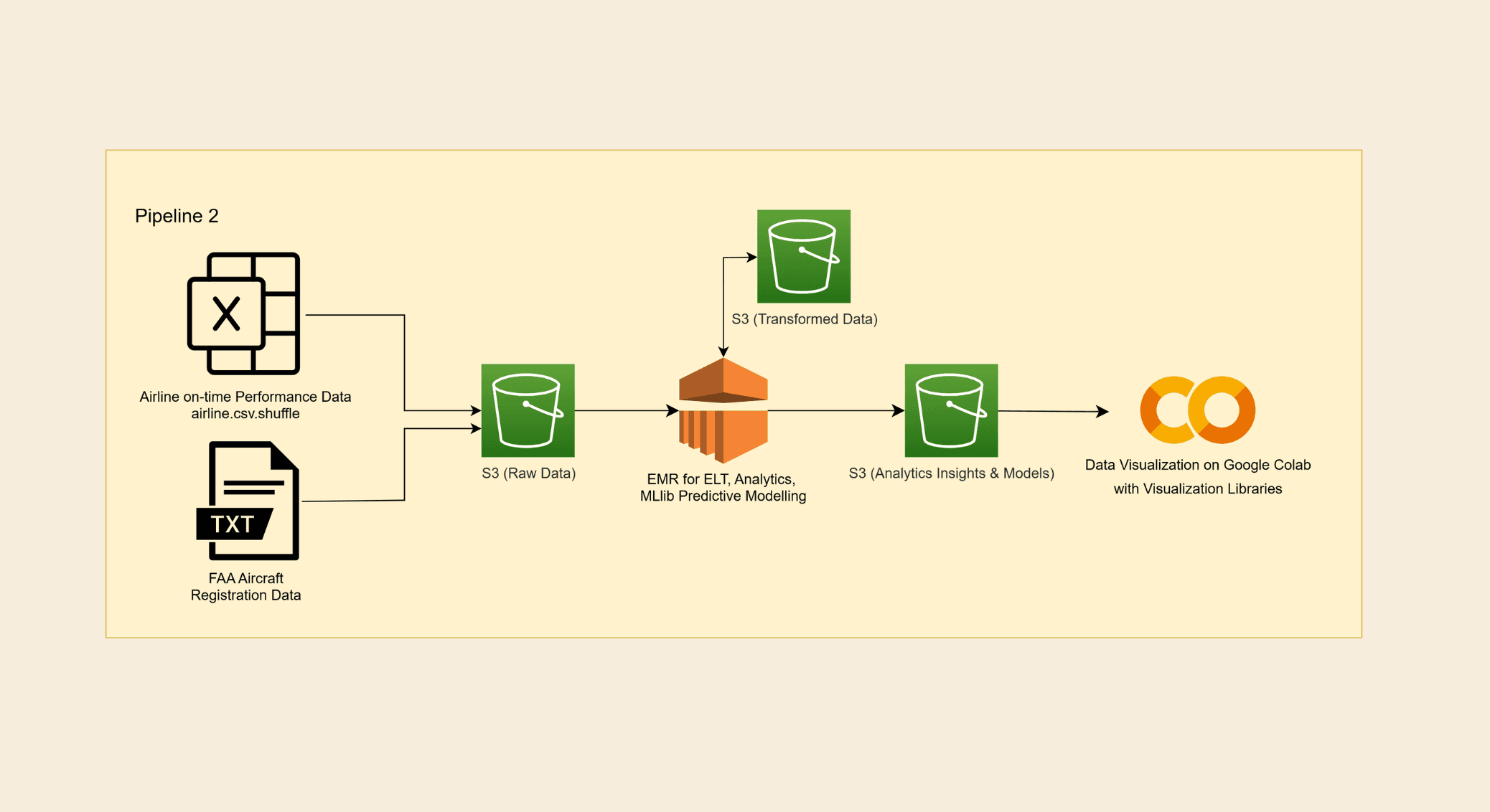
The solution architecture leaned heavily on AWS managed services, evolving from Glue-based ETL into a robust, EMR-centric analytics pipeline with notebook-driven development.

• Amazon S3
  Served as the central data lake for:

  • Raw airline on-time performance CSVs.
  • FAA registry files (MASTER / ACFTREF).
  • Partitioned Parquet tables of enriched flight chains and downstream analytics outputs.

• AWS Glue

  • Used for initial data cataloguing, schema inference and partitioning.
  • It played a central role in the airport congestion pipeline (joining flight data with weather) and provided the Glue Data Catalog, which acted as the shared metastore for both Glue jobs and EMR notebooks.

• AWS EMR

  • Handled the heavy transformation and analytics workloads for aircraft-level propagation: chain detection, metric computation, and ML modelling.
  • Migrating this work from Glue to EMR gave us more control over cluster sizing and runtime, letting us scale clusters only when needed and shut them down when idle.

• EMR Studio + Notebooks

  • EMR Studio was the main development environment for PySpark notebooks.
  • This notebook-first workflow made it easy to iterate on complex UDFs, inspect intermediate DataFrames, and debug chain logic and joins.

• Amazon Athena

  • Used for quick SQL-based sanity checks on S3 tables (row counts, joins, sampling) without needing to spin up an EMR cluster.

• Spark MLlib on EMR

  • Used for training Gradient Boosted Trees and Multilayer Perceptron classifiers for the two-stage cascade prediction model.
  • Running MLlib directly on the EMR cluster meant the model could be trained close to the data without large-scale exports.

---

Modelling Delay Propagation

1. Data Transformation on EMR

Most of the heavy lifting happened in PySpark notebooks on EMR.

Timestamp Normalisation

• Input fields were raw HHMM strings, sometimes with decimals, missing values, or overnight flights.
• We standardised them by:
  • Cleaning and left-padding ("930" → "0930", "1141.0" → "1141").
  • Treating "0000" and empty strings as missing.
  • Detecting overnight legs (e.g. depart 23:00, arrive 01:30 next day) and shifting the arrival date by +1 day.

Data Quality Pipeline

• Filled missing delay fields, deduplicated rows, and removed only obvious outliers, preserving ~99% of rows for analysis.

Chain Detection

• Flights are grouped by tail number and sorted by departure time.
• A 6-hour gap threshold is applied:
  • If the gap between an arrival and the next departure exceeds 6 hours, a new chain (operational “shift”) begins.
  • Rationale: aligns with FAA duty regulations; experiments with 4 hours were too fragmented, while 8 hours was too loose.

This produced stable flight chains that reflect realistic aircraft and crew shifts rather than arbitrary daily cuts.

Propagation Metrics

For each leg in a chain we computed:

• prop_depth: length of consecutive downstream delays, respecting turnarounds.
• flights_to_recovery: number of legs until the chain returns to “on-time” behaviour.
• delay_amplification: how much delay grows (or shrinks) across successive legs.

The resulting table, chains_with_metrics, was written to partitioned Parquet in S3 for fast reuse in analytics and modelling.

2. Joining FAA Enrichment

A second set of notebooks joined FAA aircraft metadata to the subset of “cascader” aircraft (those with significant propagation metrics):

• Normalised tail numbers and applied two-phase matching to reconcile operational N-numbers with FAA records.
• Used ACFTREF codes to decode into model families (e.g. 737, A320, EMB regional jets).

The output faa_enriched_cascaders feeds aircraft-age and model-level analysis.

3. Predictive Modelling – Two-Stage Cascade Prediction

A single model struggled with the extreme class imbalance (≈95% non-cascades vs 5% cascades), so we adopted a two-stage strategy:

1. Stage 1 (Binary) – Will this flight cascade?

   • Label: whether downstream legs show propagation beyond a chosen threshold.
   • Handles the full, highly imbalanced dataset using class weights so that rare cascades are still learnable.
   • Operational role: fast real-time screen — “is this leg likely to cause trouble?”

2. Stage 2 (Multi-class) – If it cascades, how many legs? (1, 2, 3+)

   • Trained only on the 5% of flights identified as cascades.
   • This subset is much more balanced (~60% one-cascade, ~25% two-cascade, ~15% three+), making Macro F1 a natural evaluation metric.
   • Operational role: deeper analysis for the small subset of risky flights — “how bad will it be?”

Models

For both stages we experimented with:

• Gradient Boosted Trees (GBT) for strong, tabular-style performance on engineered features.
• Multilayer Perceptron (MLP) to test a simple neural baseline on the same feature set.

In combination, Stage 1 filters out the easy non-cascade cases, and Stage 2 focuses model capacity on meaningful distinctions between different cascade severities.

---

Key Findings

1. Problematic Aircraft, Risk Scores & Risk Quadrants

We aggregated propagation metrics by tail number, computed composite risk scores, and segmented tails into risk quadrants:

• Thresholds like propagation depth ≥ 1.0 and propagation rate ≥ 25% were used to flag severe, frequent cascaders.
• Most aircraft are low-risk (≈86.4%), while only ~0.4% fall into a “critical” category—but those few have disproportionate network impact.

To make this more interpretable for operations teams, each aircraft is placed into one of four risk quadrants:

• 🔴 CRITICAL – high propagation rate and high depth (frequent and long cascades)
• 🟠 HIGH_RATE_LOW_DEPTH – frequent but shallow cascades
• 🟡 LOW_RATE_HIGH_DEPTH – rare but deep cascades
• ✅ LOW_RISK – low rate and low depth (best performers)

This supports a focused intervention strategy: schedule buffers, maintenance checks, or special handling for a small set of high-risk tails instead of treating all aircraft equally.

2. Turnaround Time as an Operational Lever

We bucketed planned turnarounds and analysed propagation metrics by bucket:

• Longer planned turnarounds → more variable but less harmful in terms of cascading:
  • Average propagation depth trends toward ~0, as chains have time to recover.
  • Cascade rate decreases and absorption increases.

Operationally: giving tight turnarounds to already risky aircraft is a bad idea; allocating extra buffer to them is a simple, high-leverage fix.

3. Fleet Utilisation

By grouping aircraft by utilisation band:

• Lower-utilisation aircraft show significantly lower propagation depth.
• Propagation and absorption rates don’t move much with utilisation, but the length of cascades does.

So high utilisation itself isn’t always bad—but when aircraft are both highly utilised and delay-prone, cascades become longer and harder to recover from.

4. Time of Day: When Delays Compound

Time-of-day analysis shows:

• During the day (especially bank periods), average propagation depth increases: more flights, longer chains, and more opportunities for delay to spread.
• At night, average absorption increases as lighter schedules provide natural slack for recovery.

This suggests that morning and late-afternoon waves deserve stricter control on tight connections and high-risk tails.

5. Best vs Worst Carriers

Even with the same infrastructure:

• Best performers (e.g. Hawaiian Airlines, Aloha) exhibit low propagation and high absorption rates.
• Worst performers (e.g. ExpressJet) show the opposite pattern.

This highlights that operational practices (crew planning, maintenance, schedule design) matter as much as physical constraints.

6. Aircraft Age & Model (FAA Enriched Analytics)

Using the FAA-enriched dataset:

• Age: Propagation depth, rate and absorption are broadly similar across age buckets — we explicitly looked for “older aircraft are worse” patterns and found little evidence; delays seem driven more by operations than by aircraft age alone.
• Model / type: We searched for specific aircraft families that were clear outliers. While some models show slightly higher depth or rate, there is no single “smoking gun” type; results are often limited by sample sizes in certain configurations.

Overall, the FAA analysis suggests that how aircraft are scheduled and operated carries more weight than their age or model alone.

---

Methods & Implementation (Technical Appendix)

Data Ingestion & Storage

• Raw flight data (airline OTP) and FAA registry files are stored in S3 under separate prefixes for raw/ and processed/.
• Glue crawlers infer schemas and register tables in the Glue Data Catalog, which serves as the unified metastore for both Glue ETL jobs and Spark on EMR.
• The chain-processing notebook writes a partitioned Parquet table chains_with_metrics to S3, using data_month=YYYY-MM partitions for efficient reads.

Compute Layers

• Glue Jobs (Q1 + shared ETL)

  • Batch ETL for flight and weather data, and initial transformations for congestion windows.
  • Good for scheduled jobs and batch-only pipelines.

• EMR Clusters (Q2, on-demand analytics)

  • Multi-node EMR clusters (backed by general-purpose m5 instances) run PySpark workloads for:
    • Chain building and propagation metric computation.
    • FAA enrichment joins.
    • Model training (GBT, MLP) for the two-stage cascade predictor.
  • Clusters are ephemeral: spun up for heavy work, then terminated once outputs are written to S3.

• EMR Studio + Jupyter Enterprise Gateway

  • EMR Studio provides user workspaces; notebooks connect to EMR clusters via Jupyter Enterprise Gateway.
  • Spark sessions are configured to use the Glue Data Catalog as the Hive metastore, so the same table definitions can be queried from Glue, EMR and Athena.

Caching Strategy

• A simple configuration flag controls whether a notebook:
  • Recomputes chains_with_metrics end-to-end, or
  • Reloads cached Parquet from S3 (LOAD_FROM_S3 = True) for fast experimentation.
• This approach:
  • Keeps repeatable, versioned “gold” tables in S3.
  • Avoids paying the full Spark cost for every exploratory notebook run.
  • Makes it easy to plug new analysis or visualisation notebooks into the existing pipeline.

Notebook Organisation

The project codebase was organised into two main tracks:

• Airport Congestion Track: Focused on weather ingestion (local + Lambda/Open-Meteo) and airport-level congestion windows.
• Aircraft Propagation Track (the focus of this post):
  • Chain-based analysis (EMR): chain building, metrics, FAA joins, and S3 caching.
  • Visualisation: risk quadrants, tail-level dashboards, and operational slices (turnaround, utilisation, time-of-day, carrier, age, model).
  • Two-stage ML modelling: feature engineering and training of the Stage 1/Stage 2 cascade predictors.

---

Conclusion

This project demonstrated how a carefully designed big-data pipeline on AWS can move from raw CSVs to actionable tail-level risk scores.

From an engineering perspective, the AWS-first architecture (S3, Glue, EMR, Athena, Spark/MLlib) made it feasible to work with multi-gigabyte datasets, chain-level computations, and iterative modelling without over-provisioning resources. Transitioning from Glue jobs to EMR notebooks for the aircraft-level analysis gave us better cost control, more flexibility, and faster iteration loops.

From a business perspective, the key takeaway is that a small fraction of aircraft behave as network multipliers. Targeting them with tailored buffers or schedule changes can yield outsized gains. We also found that turnaround time and time of day are controllable levers that meaningfully change propagation dynamics, and that operations (scheduling, utilisation, maintenance) explain more of the cascades than hardware alone.